POSTS
Building Models to Predict Strictly Dance Scores
Now that in the previous post I’ve defined the goal of our model (predict Strictly scores out of 40 for the upcoming week!) and defined teaching and testing inputs and labels from the data, it’s time to build some models!
Setting up models
I’ve decided to compare the performance of three different regressors. One is a random forest regressor (RandomForestRegressor from sklearn.ensemble) and two are different gradient boosting regressors (GradientBoostingRegressor from sklearn.ensemble, and XGBRegressor from xgboost).
I set up all three models as Pipelines in sklearn with the preprocessor defined as in the previous post.
I first tried out the models using a single set of parameters, fit them to the training set, and checked their training and test set scores. For example:
# gradient boosting regressor, gbr
est = GradientBoostingRegressor(n_estimators=100, learning_rate=0.1,
                                max_depth=1, random_state=0, loss='ls')

gbr = Pipeline(steps=[('preprocessor', preprocessor),
                      ('regressor', est)])

gbr.fit(training_inputs, training_classes)

print("unoptimized results:")
print("training set score: %.3f" % gbr.score(training_inputs, training_classes))
print("testing set score: %.3f" % gbr.score(testing_inputs, testing_classes))
The other regressors are set up similarly.
Parameter optimization via grid search
However, to try to improve the performance of all the models, I wanted to improve the parameters! In all cases, I used a grid search in which two model parameters were varied to find the best performance. The grid search was performed using the same cross-validation for all three models: a k-fold cross-validation with k=10, making sure to include shuffled sampling. (Since the data is passed in as an ordered timeseries, I particularly didn’t want different splits to only sample particular series!) The prediction score was evaluated using r-squared coefficients of determination.
For the gradient boosting regressor and the xgboost regressor, I allowed the number of estimators and the learning rate to vary. For the random forest regressor, I allowed the number of estimators and maximum features to vary.
After running the grid search, each GridSearchCV instance then provides a best_estimator_ attribute containing a refitted version of the regressor that uses the parameters that gave the best score. (Not shown here, I also followed the example of Randal S. Olson in visualizing the grid search results to see how sensitive the model accuracy is to the searched range of parameters. I used this to help determine at what point expanding the range of the grid search is not meaningfully helpful in improving accuracy.)
Example grid search:
learning_rates = np.array([0.01, 0.1, 0.5])
n_estimators = np.array([50,100,200,500,1000,2000,5000])

parameter_grid = {'regressor__n_estimators': n_estimators,
                  'regressor__learning_rate': learning_rates,
                  }

grid_search = GridSearchCV(gbr,
                           param_grid=parameter_grid,
                           cv=cv_shared)

grid_search.fit(all_inputs, all_labels)

gradient_boosting_regressor_best = grid_search.best_estimator_

print('Best score: {}'.format(grid_search.best_score_))
print('Best parameters: {}'.format(grid_search.best_params_))
Comparing optimized model performance
Finally, I can compare the performance of the three models with a box-and-whisker plot that compares the distribution of accuracy scores from the 10-fold cross-validation.
xb_df = pd.DataFrame({'accuracy': cross_val_score(xgbr_optimized, all_inputs, all_labels, cv=cv_shared),
                       'regressor': ['XGBoost'] * 10})
dt_df = pd.DataFrame({'accuracy': cross_val_score(gradient_boosting_regressor_best, all_inputs, all_labels, cv=cv_shared),
                      'regressor': ['Gradient Boosting'] * 10})
rf_df = pd.DataFrame({'accuracy': cross_val_score(rfr_best, all_inputs, all_labels, cv=cv_shared),
                      'regressor': ['Random Forest'] * 10})
all_df = xb_df.append(dt_df).append(rf_df)

sns.boxplot(x='regressor', y='accuracy', data=all_df)
sns.stripplot(x='regressor', y='accuracy', data=all_df, jitter=True, color='black')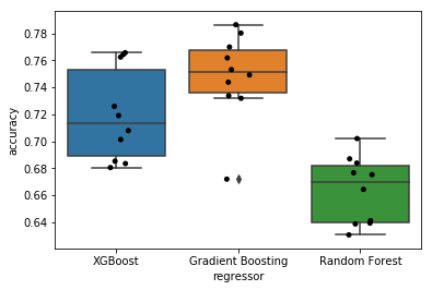
Plot: box-and-whisker plot comparing three models
Overall, the r-squared score range of 0.6 to 0.8 doesn’t seem that bad! Comparing the three models, you can see different amounts of variability in accuracy across the cross-validation splits. However, taken overall, the gradient boosting regressor seems to have the highest accuracy, at least when optimizing over the grid searches that I performed.
So, now that we have the models, it’s time to make some predictions about scores in a new episode, and evaluate how they turned out. That will be next!
And remember, keeeeeeeeeeeeep data-ing!
Note: thanks to Randal S. Olson for his “An example machine learning notebook”, to which the above analysis is heavily indebted.