POSTS
Week 4 Score Evaluation
The judges have their scores! Let’s see how they compare to the Week 4 predictions.
| celebrity | professional | dance | fan | gbr | xgbr | rfr | actual |
|---|---|---|---|---|---|---|---|
| Ashley Roberts | Pasha Kovalev | Tango | 36 | 32 | 33 | 28 | 32 |
| Charles Venn | Karen Clifton | Salsa | 25 | 24 | 24 | 25 | 25 |
| Danny John-Jules | Amy Dowden | Viennese Waltz | 29 | 29 | 30 | 27 | 27 |
| Faye Tozer | Giovanni Pernice | Rumba | 36 | 30 | 28 | 29 | 29 |
| Graeme Swann | Oti Mabuse | Jive | 30 | 22 | 25 | 23 | 26 |
| Joe Sugg | Dianne Buswell | Cha-cha-cha | 28 | 26 | 28 | 25 | 26 |
| Kate Silverton | Aljaž Skorjanec | Samba | 28 | 25 | 26 | 26 | 20 |
| Katie Piper | Gorka Márquez | Jive | 21 | 17 | 17 | 20 | 18 |
| Lauren Steadman | AJ Pritchard | Quickstep | 25 | 23 | 24 | 26 | 25 |
| Dr. Ranj Singh | Janette Manrara | Paso Doble | 25 | 24 | 26 | 25 | 27 |
| Seann Walsh | Katya Jones | Charleston | 30 | 23 | 23 | 23 | 28 |
| Stacey Dooley | Kevin Clifton | Foxtrot | 30 | 27 | 27 | 25 | 33 |
| Vick Hope | Graziano Di Prima | Quickstep | 28 | 25 | 26 | 25 | 29 |
A reminder:
fanis a Strictly super-fan’s independent predictionsgbris a gradient boosting regressor, previously selected as the best-performing model and the official prediction to compare to a human expertxgbris an XGBoost regressorrfris a random forest regressor
Focusing on the fan and ‘best model’ gradient boosting predictions for a moment, we can also view the results graphically:
import seaborn as sns

with sns.plotting_context('poster'):
    sns.pairplot(df, x_vars=['fan','gbr'], y_vars=['actual'],
                 hue='celebrity', height=6)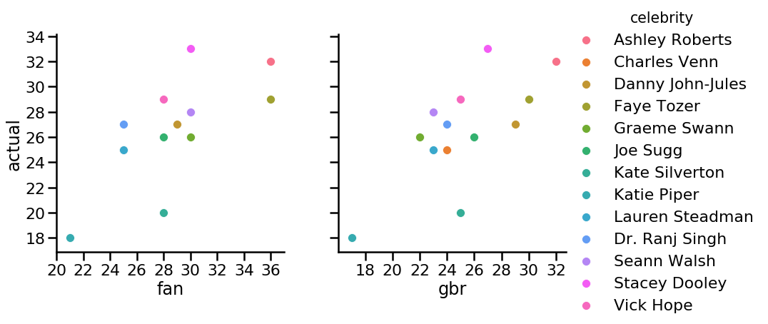
Plot: scatter plots comparing predicted and actual scores for Week 4
Not bad, overall, though certainly a few surprises! Notably, some of the biggest surprises—a low score by Kate and Aljaž, and Stacey and Kevin sitting at the top of the leaderboard—seemed more or less equally surprising to both the expert and the model.
I’ve tried using different metrics to evaluate more quantitatively the predictions. As we’ll see, the quality of a prediction depends on the metric I use.
Number of exactly correct scores
for predict in ['fan','gbr','xgbr','rfr']:
    num_right = (df[predict]==df['actual']).sum()
    print('{} : {}'.format(df[predict].name, num_right))
results in
fan : 2
gbr : 2
xgbr : 0
rfr : 3
The expert and ‘best model’ both got a pair of scores exactly right (a different pair, in each case). The random forest regressor had the most exactly correct, but I’m not sure if that is convincing evidence for the random forest’s predictive power. The random forest predicted lots of middling scores, so it’s not all that surprising that someone scored in that middling range.
Root mean square error (RMSE)
for predict in ['fan','gbr','xgbr','rfr']:
    rmse = mean_squared_error(df['actual'], df[predict])**0.5
    print('{} : {:.1f}'.format(df[predict].name, rmse))
gives
fan : 3.7
gbr : 3.3
xgbr : 3.1
rfr : 3.7
R-squared (coefficient of determination) score
for predict in ['fan','gbr','xgbr','rfr']:
    r_2 = r2_score(y_true=df['actual'], y_pred=df[predict])
    print('{} : {:.2f}'.format(df[predict].name, r_2))
gives
fan : 0.13
gbr : 0.33
xgbr : 0.39
rfr : 0.15
Conclusions
Overall, the gradient boosting regressor I chose to make my “best” model prediction did at least as well at predicting Week 4 scores as a Strictly fan! Both got two scores exactly right, while the gradient boosting regressor also achieved a somewhat lower RMSE and larger r-squared value.
Overall, the XGBoost regressor made the best predictions, in terms of minimizing the RMSE and maximizing the r-squared. This is in contrast with the cross-validation results, in which on average the plain gradient boosting scored higher r-squared values when the entire 16 series of Strictly data was available. I can think of two possible explanations for the discrepancy:
- For this particular prediction, it was random chance that XGBoost did better. This is certainly plausible because the distributions of r-squared scores for the two models in the cross-validation did overlap.
- The XGBoost model does a somewhat better job at this kind of extrapolation problem, in which less is known about the celebrities, compared to the plain gradient boosting model.
Another interesting point is that though XGBoost did best taken as a whole, it didn’t get any scores exactly right, whereas the random forest did the worst overall, but happened to get three scores exactly right. This highlights the importance of thinking carefully about how to evaluate model performance.
And finally, all r-squared scores are quite a bit smaller than the cross-validation results. Again, this is probably because the amount of data available for the Series 16 dancers (only three previous weeks, including an often challenging first week) was much smaller than the amount of data typically available for a given celebrity in the full training set.
I plan to make another round of predictions for Week 5 scores. Based on the results from Week 4, I will use the XGBoost regressor as the model to put head-to-head against the expert fan prediction. One added wrinkle is a guest judge will replace Bruno. Though I’ll retrain the models with the Week 4 results added, will the model performance suffer by not accounting for the loss of everyone’s favorite Bananarama-choreographing gesticulator?

We’ll have to see on Saturday. But until then, keeeeeeeeeeeeeeep data-ing!