POSTS
Week 5 Scores: A Tough Week to Predict
Lots of surprises during Week 5 of Strictly Series 16!
Not from this week, but still a surprise.
To predict Week 5 Strictly results, I retrained the same three models as I used previously for Week 4, adding in the Week 4 results as additional model inputs. Since this represents a 33% increase in available data about the performance of this series’ celebrities, I was hopeful the model predictions would improve. However, the week also included two factors that threatened to befuddle the models:
- Bruno was off for the week, and would be replaced by former Dancing with the Stars champion and Fresh Prince of Bel-Air actor Alfonso Ribeiro (—and now I also see on his Wikipedia page current host of America’s Funniest Home Videos, which apparently has decided to thumb its nose at the internet and trudge on).
- The new “couple’s choice” category had its debut, with two routines in styles never before performed on the show (contemporary and “street/commercial”).
Despite these warning signs, I still went ahead and predicted a score for each routine. Because it did the best last week, I decided to use the XGBoost regressor predictions as the “official” submission, though cross-validation performance of the plain gradient boosting model appeared on average slightly better than XGBoost, the same as last time.
Additionally, an expert Strictly fan again was willing to share their predicted scores as a point of comparison, for which I am thankful!

Aljaz: also thankful.
I’ve tabulated the predictions and actual scores for Week 5:
| partners | dance | fan | gbr | xgbr | rfr | actual |
|---|---|---|---|---|---|---|
| Ashley and Pasha | Rumba | 31 | 30 | 32 | 26 | 36 |
| Charles and Karen | Street/Commercial | 28 | 25 | 23 | 25 | 36 |
| Danny and Amy | Jive | 26 | 26 | 29 | 25 | 37 |
| Faye and Giovanni | Foxtrot | 35 | 32 | 31 | 29 | 33 |
| Grame and Oti | Tango | 27 | 24 | 23 | 23 | 29 |
| Joe and Dianne | Waltz | 30 | 28 | 30 | 27 | 29 |
| Kate and Aljaz | Viennese Waltz | 31 | 26 | 29 | 28 | 26 |
| Lauren and AJ | Contemporary | 30 | 23 | 23 | 24 | 24 |
| Ranj and Janette | American Smooth | 25 | 26 | 27 | 26 | 25 |
| Seann and Katya | Quickstep | 28 | 23 | 22 | 23 | 24 |
| Stacey and Kevin | Samba | 27 | 26 | 27 | 25 | 33 |
| Vick and Graziano | Cha cha cha | 28 | 23 | 26 | 25 | 20 |
I made a few charts to visualize the scoring.
First, a scatter plot to see how predictions compared to actual scoring:
with sns.plotting_context('talk'):
    sns.pairplot(df,x_vars=['fan','xgbr'],y_vars=['actual'],
                 hue='partners',height=4)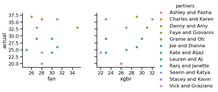
Compared to last time, you can see both the expert prediction and the model had a very difficult time predicting scores with a high degree of accuracy. To look at this more quantitatively, I calculated the same measures as last time:
print('number exactly correct:')
for predict in ['fan','gbr','xgbr','rfr']:
    num_right = (df[predict]==df['actual']).sum()
    print('{} : {}'.format(df[predict].name, num_right))

print('------')

print("root mean square error")
for predict in ['fan','gbr','xgbr','rfr']:
    rmse = mean_squared_error(df['actual'], df[predict])**0.5
    print('{} : {:.1f}'.format(df[predict].name, rmse))

print('------')

print('r-squared coefficient of correlation:')
for predict in ['fan','gbr','xgbr','rfr']:
    r_2 = r2_score(y_true=df['actual'], y_pred=df[predict])
    print('{} : {:.2f}'.format(df[predict].name, r_2))
resulting in:
number exactly correct:
fan : 1
gbr : 1
xgbr : 0
rfr : 1
------
root mean square error
fan : 5.7
gbr : 5.5
xgbr : 5.6
rfr : 6.6
------
r-squared coefficient of correlation:
fan : -0.14
gbr : -0.05
xgbr : -0.09
rfr : -0.48
On all counts, the predictions were less accurate than last time. In fact, the r-squared values were near-zero or somewhat negative, implying no correlation (or even an anti-correlation!) between the predicted and actual scores.
Once again, the gradient boosting regressors performed better than the random forest regressor, though this time the plain gradient boosting was ever-so-slightly better than the XGBoost. The better performance of XGBoost last week may have been just random, since the cross-validation performance of the two weren’t all that different. The prediction accuracy of those two models were competitive with the expert fan.
I also plotted the residuals:
points = ['x','.','+','_']
with sns.plotting_context('talk'):
    for point, predict in zip(points, ['fan','gbr','xgbr','rfr']):
        resid = df[predict]-df['actual']
        plt.plot(df['actual'],resid, point, label=predict, alpha=0.9)
    plt.ylim(-14.5,14.5)
    plt.legend()
    plt.xlabel('actual score')
    plt.ylabel('residual')
    plt.title('Week 5 score residuals')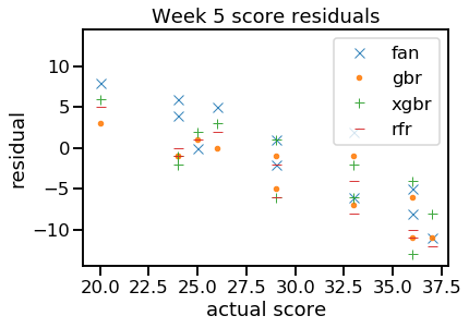
The residual plot shows us there was a definite trend in how the predictions were wrong. In all cases, the predictions overestimated the low scores and underestimated the high scores.
It’s not all that surprising this is the way in which the predictions are inaccurate. A score of 20 is low at this point in the competition; it’s more plausible to guess the partnership with the 20 would have scored 5 or so points higher than even lower. Similarly, a guess that’s off by 5 or 10 points of a score actually in the high 30s must have been an underestimate, since it’s impossible to score higher than 40.
The magnitude of the underestimates of the high scores tended to be larger, likely because there were some very high scores from somewhat unexpected dances: Charles and Karen’s couple’s choice street dance, and Danny and Amy’s aviation-themed jive.
A histogram (with kernel density estimates added—thanks, seaborn!) illustrates a consistent point. The distribution of actual scores was broader than any of the predictions:
with sns.plotting_context('talk'):
    for predict in ['fan','gbr','xgbr','rfr','actual']:
        sns.distplot(df[predict], label=predict)
    plt.legend()
    plt.title('Week 5 score distributions')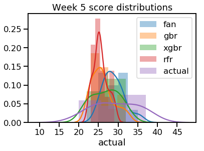
So, overall a tough week to predict! I think it’s clear why, though—many of the scores this week seemed surprising based on how celebrities had done in the past. It also didn’t help the machine learning models they were thrown situations for which no data existed (Bruno substitute, new types of dances).
I’ll have to see whether next week, Halloween Week on Strictly, will go any better. It may be spooky, but hopefully there won’t be too many scary surprises for the models!
Judges: ready.
And remember, keeeeeeeeeeeep data-ing!